Control procedure of adjustment

To control our routines of curve fitting of light, we used the close supernovæ published (hamuy1996c & riess1999).

The adjustments of the lightcurves were carried out by the groups of the HIZSN and SCP to make their measurement of cosmology (riess1998, perlmutter1999, tonry2003 & knop2003).

In the continuation, we will compare the results obtained by knop2003 with those of this analysis.

The analysis of the lightcurves made by knop2003 rests on the adjustment of the owners of lightcurves built by goldhaber2001, which have by definition a factor of stretching equal to 1.

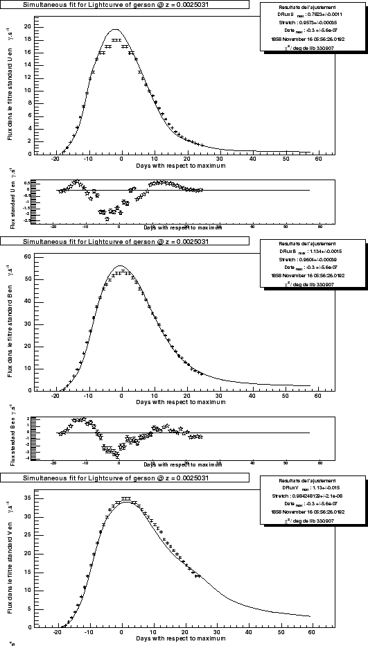
We thus used the owner out of B to express the value of the factor of stretching resulting from our analysis according to the true `` '' factor of stretching. Figure 9.8 shows the result of the adjustment of the owner, it gives us:

$$s_{U} = 0.957~ s^U_{standard}$$ (9.10)

$$s_{B} = 0.960~ s^B_{standard}$$ (9.11)

$$s_{V} = 0.984~ s^V_{standard}$$ (9.12)

with $s^V_{standard}$ respectively values of factor of stretching defined for the owner of goldhaber2001.

This figure shows moreover, that fluxes to the maximum for our model are slightly higher out of U and out of B This should not have incidence in theory, all measurements of cosmology will be made by using curve fittings of light with the same model.

Figure 9.8: Comparison of the models of lightcurve of knop2003 and our our simulator in flux. From top to bottom, we consider standard bands UBV.

The lightcurves show a relatively good agreement however. Let us see how into term of estimate of the parameters of the curves of light that is translated.