Construction of the effective filters

The effective filters $T_{eff}$ are defined like:

$$T_{eff}(\lambda) = T_f(\lambda) T_{atm}(\lambda) T_{opt}(\lambda) Qe(\lambda)$$ (9.1)

The construction of the effective filters thus requires to know the various transmissions of each part of the system of observation. The transmission of optics, the reflectivity of the mirror, the quantum effectiveness of each CCD (there can be substantial differences of one CCD to the other) and the transmission of the filters are in general given at the time of the design and the startup of the instruments by the manufacturers.

In the case of the Hubble telescope, this calibration in laboratory was made with much care. It made it possible to determine synthetic items zeros with values very close to the values determined by the standard star observation in orbit (holtzman199ä).

Unfortunately, it was not possible to join together sufficiently precise information to allow the same kind of simulation for the telescopes on the ground.

A significant effort was made to reproduce zero points of instrument CFH12K of the CFHT.

The supernovæ of this study were discovered on 2 CCDs (the CCD 4 and the CCD 10). We tried to determine the effective filters for these two CCDs

The CFH12K is made up of 12 CCDs of two different types: those of great resistivity (of which the CCD 4) and CCDs EAR (of which the CCD 10). The evaluation of the quantum effectiveness was not carried out in a systematic way for all CCDs of the mosaic, the quantum operating characteristics presented here are averages on CCDs for which there are measurements.

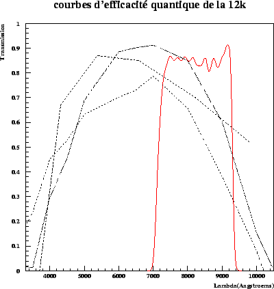
Figure 9.1 was estimated at for the CCD 4. We have for each filter, knowing items zeros except atmosphere and the transmission of the remainder of optics, considered the effectiveness quantum average in the filter (each point correspodant with this value with the average wavelength of the filter).

We see that this curve presents significant differences compared to the quantum operating characteristic of standard CCDs in the same way (those of great resistivity which correspond to the curve into dotted).

This problem is all the more critical as all the observations with this instrument were carried out in the filter I where the quantum variation of effectiveness is largest and influential much on the shape of the effective filter.

Figure 9.1: Quantum operating characteristics of the CFH12K for different CCDs compared with filter I in red. The curve in dotted line is the quantum effectiveness provided by the CFHT for CCDs of great resistivity, the curve in indent-dotted line is the curve for CCDs EAR, the curve in indent is an estimate of the quantum operating characteristic of the CCD4 (of great resistivity) starting from zero points in each filter of CFH12K (BVRI).

The various attempts to reproduce starting from these quantum operating characteristics zero points and the terms of color were not conclusive. We thus decided to measure photometry on the ground by using the standard method of calibration using zero points and the terms of color as presented in appendix A .

The majority of the points of the photometry and in particular most precise were measured with the space telescope. There are typically 2 to 3 points on the ground for 6 to 10 points taken with the space telescope. Moreover, the points measured on the ground are often the images of research of the supernovæ and present more significant photometric errors. The errors introduced by the calibration on the ground will be thus tiny.