The principal difficulty of this stage comes from the presence of artifacts like the died pixels, the cosmic ones or the satellites, which one obviously wishes to eliminate.
In addition the various components of the sums are taken under conditions which can vary. In particular, the bottom of sky (the dominant source of noise), the seeing or absorption by clouds of high altitude (cirri), can vary from one image to another in particular if they all are not acquired the same night.
It is thus desirable during this `` '' addition to give a more significant weight to the images of better quality.
To simplify the notations, we suppose in what follows that the funds of sky were withdrawn, i.e. that the images present objects on a bottom on average no one. As atmospheric absorption can vary image with image, we have:
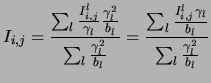 |
(7.19) |
Insofar as one has several estimates of the same quantity, one
can try at this stage to compare the values to eliminate those which
are aberrant, due for example to cosmic, a plane having crossed the
field or to the defects of the instrument. One must then compare each
one of ![]() ,
and eliminate it from the sum if it is unacceptable, while reiterating
until convergence. A limitation of this technique is that it asks to
have a relatively significant number of images, in practice at least 5
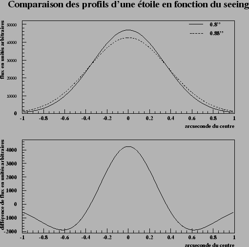
to 6 images. More serious, like figure 7.15 illustrates it ,
the variation of seeing between the images can involve the systematic
rejection of pixels on the level of the objects present on the images.
The stars see their profile completely deformed in a manner which
depends on their flux.
,
and eliminate it from the sum if it is unacceptable, while reiterating
until convergence. A limitation of this technique is that it asks to
have a relatively significant number of images, in practice at least 5
to 6 images. More serious, like figure 7.15 illustrates it ,
the variation of seeing between the images can involve the systematic
rejection of pixels on the level of the objects present on the images.
The stars see their profile completely deformed in a manner which
depends on their flux.
This problem appears in a crucial way only when one summons images of different nights, and especially if they enter subtractions then, which few programs of observation require. This is why the technique described here is largely used in the community, without putting the scientific results in danger. For us, it is the system of observation in tail, which by splitting our long integrations on 3 or 4 nights obliged us to re-examine our approach.
 |
One could limit the problem by bringing all the images to the same resolution ( i.e. with same the seeing) by convoluting each image by a core bringing them all to the same resolution as the image of worse seeing. In addition to this operation is expensive in computing times, it will downwards reduce the resolution of the images coadditionnées by levelling the quality of the images. But it is clear that if one wishes to set up a rejection of the intruder as indicated higher, it is necessary to homogenize qualities of image.
We implemented another approach, which consists in identifying the defects of the individual images indépendemment from/to each other, so as to mask the corresponding pixels during the addition. It is a rather heavy approach, because it requires to develop specific algorithms of detection for each type of defect.
As we saw before, we have the charts already labelling the dead pixels and the pixels of saturated stars. We want to now build the images containing the pixels reached by the cosmic ones and those by satellites.