Measurements of distances from luminosity: practice

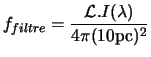
The measurement of the intrinsic luminosity of an object is in general expressed like its magnitude measured at a distance from $\lambda$ of the intensity of the object, its flux in a filter is expressed:

$$f_{filtre} = \frac{{\cal L}.I(\lambda)}{4\pi(10 {\rm pc})^2}$$ (2.17)

by using the definitions magnitudes given in appendix A , one a:

$$m_{filtre} = -2.5\log_{10}(F(filtre)) + 2.5 \log_{10}(f_0(filtre))$$ (2.18)

While using, these definitions, it comes:

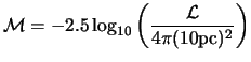$${\cal M} = -2.5 \log_{10}\left(\frac{{\cal L}}{4\pi (10 {\rm pc})^2}\right)$$ (2.19)

One can finally reexpress the magnitude of our object like:

$$m(z) = {\cal M} +25 -5 \log_{10}(H_0) + 5\log_{10}({\cal D}(z,\Omega_{\rm M}, \Omega_{\rm X}))$$ (2.20)

with ${ \cal D } = H_0d_L$.

By considering redshifts small in front of 1 and by using equation 2.11 , this relation can récrire:

$$m(z) = {\cal M} +25 + 5\log_{10}(cz) -5 \log_{10}H_0+1.086(1-q_0)z$$ (2.21)

The diagram built while carrying the magnitude of the object in ordinate and the redshift in X-coordinate is called diagram of Hubble. In illustration, the diagram of Hubble obtained thanks to the measurement of an about sixty supernovæ of the Ia type within the framework of the Supernovas Project Cosmology.

Figure 2.3: Diagram of Hubble for 60 supernovæ of the type Ia. This figure shows in particular the lifting of degeneration between the various models of universe for redshifts beyond 0.5.

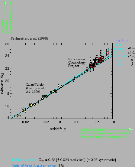In practice, one takes these measurements by comparing a batch of standard candles close with a batch to remote standard candles. For the two batches, the terms depending on the intrinsic luminosity of the object and the constant of Hubble are identical.

The comparison of the distances from the close and remote objects thus makes it possible in practice to completely uncouple measurements from ( $\Omega_{\rm M_0}, \Omega_\Lambda$) from the constant of Hubble it , the part of the diagram with great redshifts (around 0.5) makes it possible to raise the degeneration between the various sets of cosmological parameters. In the field of the small shifts towards the red, relation 2.21 shows that the relation between the magnitude and the shift towards the red is logarithmiquement linear. The extrapolation of this relation makes it possible to measure a linear combination intrinsic magnitude of the object and constant of Hubble. The knowledge of the intrinsic luminosity thus allows in theory a measurement of the constant of Hubble.

It is partly this technique which was put in uvre for the determination of the constant of Hubble within the framework of the HST Key Project (freedman2001) that we presented in the first chapter. The results are summarized in table 1.1 .

The standard candles are thus in theory an extremely powerful tool to force the cosmological parameters: the constant of Hubble with small redshifts (around 0.1) and the reduced densities with great redshift.

However, there are several difficulties. First is that it is necessary to find objects whose luminosity allows the measurement of a flux for great shifts towards the red. It is the case in practice only for the galaxies and the supernovæ. We will see in the continuation why the supernovæ and especially, a particular class of supernova allows this kind of measurement. The galaxies were used since Hubble to build diagrams of Hubble .

A certain number of other difficulties come to affect measurements. They are related mainly to the conditions of observations, in the continuation we present the principal corrections and biass related to measurements of flux.