Propagation of zero points with the photometric references

The procedure of coaddition does not make it possible to directly use the total duration of the image. In particular, can return in the coaddition of the images presenting a certain absorption.

We thus will use the images of photometric references primary. The propagation of zero points is made by using the photometric reports/ratios of the objects present on the two images.

The method simplest to put in uvre, is to use the catalogues of photometry of the images to consider the report/ratio photometric. However, the methods of calculation of flux (by SExtractor or DAOphot) can introduce biass related to the methods of estimate of fluxes. In particular, SExtractor flux used is a flux isophotal (where one takes into account only the pixels above a certain threshold), fluxes on the major images are thus in theory larger.

The estimate of flux by using DAOPHOT rests on a good knowledge of the PSF in the image. As we saw, we are sometimes brought to coadditionner of the very different images of seeing, thus introducing significant distortions into PSFs. There can thus there too be a systematic bias between the fluxes measured on the individual images and fluxes on the coadditionnées images.

We have thus to decide to use an estimate of a core of convolution allowing to pass from the individual image to the coadditionnée image. The integral of the core will be the photometric relationship between the two images.

This method comprises several advantages:

1. It takes into account a possible evolution of the bottom on the image.

2. It uses all the pixels of the objects, which makes it possible in particular to use the galaxies.

3. It brings the two images to the same resolution.

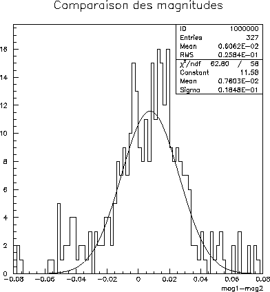
Figure 8.29 shows the histogram of the differences in magnitudes for the objects of two coadditionnées images taken with the CFHT. We see that the propagation of zero points is not biased (the average of the residuals is lower than %). the dispersion of the residuals corresponds to the photometric errors on each object. It is of the same order of magnitude as the dispersions observed for the estimates of zero points.

Figure 8.29: Comparison magnitudes obtained for two images taken with the CFH12K for different nights. Items zeros were estimated by using the method described in the text. One does not see appearing systematic biass, dispersion is mainly due to the photometric errors and are of the same order of magnitude as the precision of zero points.

Figure 8.30: Comparison magnitudes obtained for two images taken with the MOSAIC2 of the CTIO and FORS with the VLT. Items zeros were estimated by using the method described in the text. One notes a small bias of about 2% and one dispersion some 3 times more significant than for figure 8.29 . This comes from the difference between the filters used for the observations.

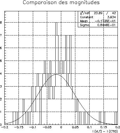figure 8.30 shows the same histogram for two different telescopes: the CFHT and the VLT. The systematic differences between the two estimates are mainly due to the differences between the transmissions of the two systems of observation.

We did not have the observations of the observations in the two filters and for the two telescopes, we thus could not study these effects according to the color of the objects observed.

Let us see however how it is possible to take account of these differences in transmissions.