 |
(8.5) |
If the bottom has a negligible contribution to the variance, one can récrire 8.4 like:
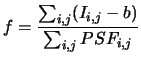
It is the definition of the aperture photometry. Its setting is practical is extremely simple, it consists in integrating the flux of the object in a ray centered on star. In practice, the ray of integration cannot be infinite (presence of other objects, minimization of the integrated noise...), the denominator thus makes it possible to make a correction for the contributions to the flux of star apart from the aperture: correction of opening . The use of this photometric estimator is not restricted in practice with great fluxes, because it does not require the precise knowledge of the PSF (the precision on uncertainties is in fact secondary, provided that they are smooth). The obvious disadvantage is the loss of optimality for weak fluxes.
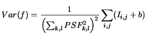
The variance of the flux estimated by aperture photometry is written:
 |
(8.6) |
 |
(8.7) |
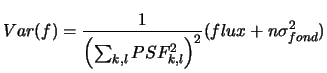
where ![]() , the fluctuations of the bottom of sky of the image.
, the fluctuations of the bottom of sky of the image.
This photometry will be used within the limit of great fluxes.