Photometry: some definitions

One understands by photometry, the estimate of the flux of an astronomical object measured using a detector of photons. This detector can take several forms (the human eye, a photomultiplier, a photographic plate, CCDs...). For more details on these various detectors to refer to sterken1992.

It generally includes/understands two stages: the measurement of the flux given by the instrument (for example, a number of electrons for CCDs and photomultipliers) and the calibration of this flux allowing to correct for the transmission and the effectiveness of the instrument.

In this part, we will detail the first stage.

All the observations of our supernovæ were made with cameras CCD, we will thus develop only this aspect of photometry.

The data are in the form of images digitalized in two dimensions. The space unit is the pixel (the positions are located according to the first pixel in bottom on the left), it contains either a number of ADU (the number of blows of ADC) or a number of photoelectrons (the number of electrons actually detected by the CCD) according to whether the image were multiplied or not by the gain. However, as we saw in the chapter of detection, none of these two units corresponds to a physical measurement, it is the stage of calibration which will make it possible to reexpress them in units of flux on the sky. The use of cameras CCD makes it possible to have a space good resolution (about the surface covered by a pixel on the sky is some tenths of a second of arc) and an ultimate photometric resolution (because the quantum effectiveness of the CCD is good or very good, and their noise of reading in general weaker than the bottom of sky).

One can regard a star as a specific signal: the profile which one observes on the images does not correspond to the real angular extension of the object. It corresponds to the impulse response of the system of observation and the atmosphere: its PSF . For the observations since the ground, the principal contribution to the spreading out of the signal of stars is the seeing (see the chapter of detection for the definition). Space sampling (i.e. size of the pixels) must in theory make it possible to distribute the image of a star on several pixels: one regards as acceptable a width has middle height from at least 2 to 3 pixels. It is in particular essential to be able to estimate the position of a star or to be able rééchantillonner an image without deteriorating the shape of stars radically. To measure the flux of a star, it is thus necessary to summon the contributions of the touched pixels.

We can thus model a star on an image as a profile $PSF_{i, j}$ (its integral being standardized to 1 if one integrates until the infinite one) multiplied by a flux F and the contribution of the light of the bottom of sky (presumedly uniform here) $I_{i, j}$ is thus:

$$I_{i,j} = f~PSF_{i,j} + b + \epsilon_{i,j},$$ (8.1)

where $\chi^2$ is written:

$$\chi^2 = \sum_{i,j} \left(\frac{I_{i,j} - (f~PSF_{i,j} +b) }{\sigma_{i,j}}\right)^2$$ (8.2)

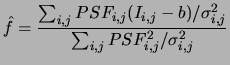
Let us suppose to simplify that flux in each pixel is expressed in photoelectrons, and that the fluctuations are Poissonnian (either in practice Gaussian because the background noise of sky is unfortunately always sufficiently large for that). The variance of the flux of a pixel is thus simply the value of flux in this pixel, that is to say:

$$Var(I_{i,j}) = \sigma_{i,j}^2 = f~PSF_{i,j} + b$$ (8.3)

The minimum of $f$ is written:

$$\hat{f} =\frac{\sum_{i,j}PSF_{i,j}(I_{i,j}-b)/\sigma_{i,j}^2}{\sum_{i,j} PSF_{i,j}^2/\sigma_{i,j}^2}$$ (8.4)

It is about the optimal estimator of the flux of a star, because he reaches the terminal of minimal variance.

This expression of the estimator of flux uses flux to evaluate the variance of the implied pixels. This autoreference can appear artificial or useless insofar as one could use the actual value of the image $I_{i, j}$ like value of the variance. It is acted in fact of an error which leads to a biased estimator of flux, because of the fluctuations pixel to pixel that the variance presents then, correlated (identical here) with the fluctuations of the image itself. In practice, flux necessary to the evaluation of the variance is calculated summarily by summoning the pixels of the object, so that the image of the variance is `` smooth ' '. If flux is weak, one can quite simply be unaware of the contribution of the object to the noise. Incidentally, it is to avoid this bias on fluxes that the charts of weight which one associates the images are not built starting from the values of the pixels of these images.

This approach of the photometry (which one simplified here by supposing the known position of the object) is called photometry of PSF. There is two borderline cases for which the estimator of flux is simplified: the limit of great fluxes where the bottom of sky can be neglected and limit of small fluxes where the contribution of the object to the noise is negligible in front of the bottom of sky. They define two extreme modes: the aperture photometry and weighed photometry .