Estimate of the parameters of the objects detected and cuts

The second stage consists in estimating in a precise way the position and flux of each detected candidate. For that, one follows the regulations of naylor1998 while using like model of PSF a Gaussian profile of width equalizes with the seeing. These two estimates make it possible to calculate a signal on more precise noise.

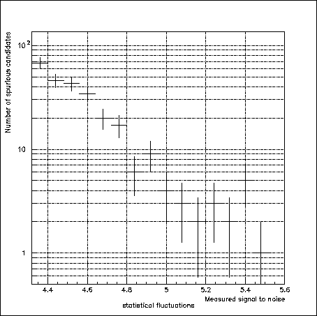
One can right now apply more restrictive cuts to the signal to noise. As figure 7.20 shows it , a cut with 5 on the signal on noise makes it possible to on average preserve only one score of candidates coming from statistical fluctuations of the bottom of sky for the equivalent of a field observed with the CFH12K.

Appear: A number of candidates coming from statistical fluctuations according to the signal on noise for 12 CCDs from $4096 \times 2048$ correspondent to the typical observation from a field with the CFH12K

Figure 7.18 shows that after the subtraction, there remain residuals of about 1 to 2% of the flux of the objects on the reference. There can thus remain residuals with signals on noise beyond the cuts on the subtraction. One thus calculates the relationship between flux on the subtraction and flux on the image of reference. A cut on this report/ratio makes it possible to eliminate all these artifacts. This cut also makes it possible to eliminate the physical objects whose variations are not very significant between the two periods of observations (active cores of galaxies or AGN, the stars variable, supernovæ of the type II).

Lastly, a certain number of mobile objects as the asteroids can pollute the fields of observations. To eliminate these objects, one carries out a separation in two batches of the images of research in order to produce two independent images of research. One withdraws the reference to these two images so as to produce two partial subtractions. The same type of detection that for the subtraction is then carried out, one seeks finally coincidences between the three subtractions. If it there be coincidence, one calculate the distance between the two detection partial, it we allow at time of inspection visual to measure the displacement of object.

Lastly, one proceeds for each candidate to an association with the object nearest on the reference. One measures in particular the distance between detection and this object.

All these cuts are summarized in table 7.1 .

Table 7.1: This table recapitulates the cuts applied during the detection of the candidates to the subtraction.

Parameters	typical cut	Functions
Signal on noise on the subtraction	> 5	eliminate the statistical fluctuations from the bottom of sky
Rate of increase in flux	> 10 to 20 %	eliminate the bad subtractions and the variable objects faiblements (AGN, other types of supernovæ, stars variable.)
Outdistance association between the partial subtractions	< 2 pixels	eliminate the asteroids
Outdistance object nearest on the reference	No cuts	informative.

The number of candidates by CCD after detection is typically ten by CCD. The majority are due to artifacts which succeeded in passing the various cuts (bad subtractions, slow asteroids, etc...). It is thus necessary to carry out a visual inspection making it possible to eliminate the defects more shouting in order to not keep but one reduced list of objects (approximately a score) which will be then observed spectroscopiquement.