Homogenisation of PSFs

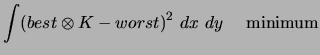
The method used is an implementation of the algorithms developed in alard1998 and alard2000. It rests on the construction of a core of convolution which makes it possible to bring the image of better quality (that of better seeing) on the second image. In practice, one seeks a core which solves the equation:

$$worst = kernel \otimes best$$ (7.22)

Where $best$ the best.

In practice, the noise does not make it possible to find solution. One thus seeks a solution by least squares:

$$\int(best\otimes K - worst)^2~dx ~dy ~~~~ {\rm minimum}$$

The core is built on the same basis of function as that proposed by Alard. It is a combination of Gaussian of variable widths multiplied by polynomials of order up to 3. This family of functions allows to take into account:

• a widening of Cur of the PSF.
• to add wings to the PSF.
• a light shift (for if required improving alignment).

The base of functions used is written in the form:

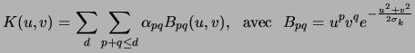$$K(u,v) = \sum_{d}\sum_{p+q \leq d}\alpha_{pq}B_{pq}(u,v),\ \ {\rm avec}\ \ B_{pq} = u^p v^q e^{-\frac{u^2 +v^2}{2\sigma_k}}$$ (7.23)

One can seek solutions with a core slowly variable in the field to be able to take into account possible variations of the PSF in the field.

The core is given using a selection of the best objects of the field (sufficient brilliant without being saturated, is a hundred objects). The core is thus estimated on labels centered on these objects.

The core is estimated by iteration, one eliminates after each turn the labels which present too significant residuals.

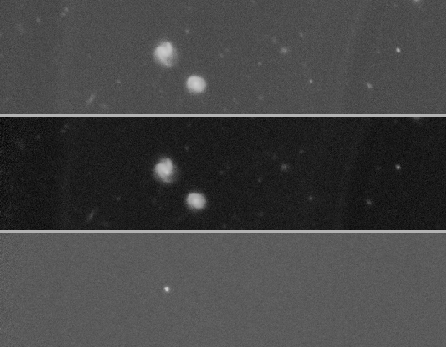
Finally, one convolutes the image of better seeing with the core thus estimated and one withdraws. For practical reasons, it is easier to express fluxes on the subtraction in photometric units of the reference (whose zero points are in general better known), the subtraction with the need is thus multiplied by the photometric relationship between the images of research and reference.

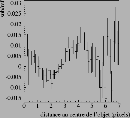
An example of subtraction is presented figure 7.18 presents the histogram of the average residuals of subtraction according to the distance at the center of the brilliant objects, reported to flux on the reference of the corresponding pixel. It remains with C$1\%$.

In all the procedure, the chart of weight of the two images is considered in particular, at the moment of the calculation of the core. The two images of weight are combined to produce a chart of weight of the subtraction which will be used at the time of detection.

Figure 7.18: Residuals of subtraction according to the distance to the centers of the objects. They are expressed like the relationship between the signal on the subtraction and the signal present on the image of reference. It is seen that the residuals of subtraction are lower than 2%.

Figure 7.19: Example of subtraction. In top, the image of reference, in the center the image of research and in bottom, the subtraction. The visible residual on the subtraction is a supernova with a redshift of 0.28. This figure shows that the residuals of subtraction on the level of the brilliant objects are not detectable with the eye.

We thus have now an image result of the subtraction of the image of research and reference and its chart of weight. It is now a question of detecting the residuals on the subtraction.