$\star$ Transformations

Pairing carried out, one can use the weaker objects to calculate a precise transformation. For that, one minimizes:

$$\sum_{i=1}^{N_{obj}} ( [u_i -T_u(x_i,y_i)]^2 +[v_i -T_v(x_i, y_i)]^2)$$ (7.18)

where $T_v$ are the transformations which make it possible to pass from one image to the other. Transformations polynômiales suffice for our needs and the adjustment is thus linear and fast. To limit the numerical problems associated with the adjustment with the polynomials, we carry out the adjustment in a reference mark or $< x_i > = < y_i > = 0$, and express then the coefficients found in the original reference mark.

When that the conversion rates are found, one calculates the residuals of transformation to eliminate the objects whose residual is too large (more than 3 times the median of the residuals). One reiterates until complete elimination of all the objects with too significant residuals.

After each iteration, the pairing of the catalogues is updated. The quality of the transformation improving, one notes that the number of associations increases.

Lastly, one compares the transformations of order 1, 2 and 3 to keep only the transformation which presents the average residual (by degree of freedom) weakest.

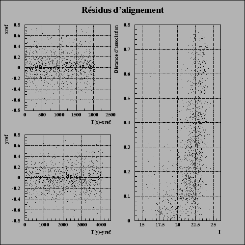
Figure 7.14 presents the residuals of transformation after this stage, they are in general better than the tenth of pixel for the images of the CFH12K.

The found transformation, it is applied to the current image. Transformations not moving the images of a whole number of pixel, one rééchantillone by using a quadratic interpolation considering 9 pixels around the point of rééchantillonage. This stage preserves the flux total of the objects but introduced correlations between close pixels.

Figure 7.14: Residuals of the geometrical transformations. The two figures on the line show the difference between the co-ordinates between the image of reference and the transform of the position of the image aligned according to the co-ordinates on the reference. Alignment makes it possible to obtain a precision of alignment of the tenth of pixel. The figure of right-hand side shows the distance between the objects on the reference and the transformed image.

All the images are thus aligned on a geometrical reference common to both times. Let us see now how they are combined to form the major images.