The images taken in the filters close to infra-red (I and Z) present sometimes fringes. In this field wavelength, CCDs are sufficiently thin to allow the interference of the light of the emission lines of molecules OH of the atmosphere, powerful beyond 800 Nm.
The figures of fringes are particular characteristics of each CCD: they schematically characterize the thickness of the CCD according to the position and are stable during the life of the CCD.
The construction of the images of fringes is done starting from the two types of charts of quantum effectiveness built for the quantum correction of effectiveness. As we saw, the light of the twilight has a primarily solar spectrum (a black body mainly) whose contributions are mainly with short wavelengths, on the other hand, the light of the night sky to strong contributions to larger wavelength. The first thus present figures of fringes much less significant.
The difference in these two images thus gives us the chart of fringes.
The second stage consists in evaluating the intensity of these fringes on the image to be corrected. Indeed, even if the figures of interferences are reproducible, their intensity very strongly depends on the quantity of light coming from the sky. Two methods are used:
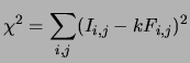 |
(7.14) |
where ![]() the chart of fringe. The minimum is reached for:
the chart of fringe. The minimum is reached for:
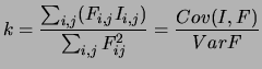 |
(7.15) |
One cannot guarantee that the illumination of the bottom of sky
is completely uniform, in particular because of the moon. To take into
account these possible variations, one adjusts simultaneously ![]() bottom polynômial:
bottom polynômial:
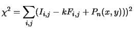 |
(7.16) |
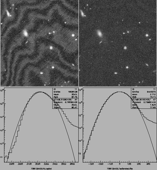
The result of this procedure is presented in figure 7.9 . One does not distinguish any more the fringes on the corrected image. The amplitude of the residual fringes which was about ![]() .
.
 |